Counting and Probability

The art of counting without counting#

Multiplication principle: independent choices multiply. A menu with 4 starters, 5 mains, 3 desserts offers 4 \times 5 \times 3 = 60 meals.

Two refined tools follow, distinguished by one question — does order matter?

\begin{aligned} \textbf{Permutations} \text{ (order matters):} \quad {}^nP_r &= \frac{n!}{(n-r)!}\\[2pt] \textbf{Combinations} \text{ (order doesn't):} \quad \binom{n}{r} &= \frac{n!}{r!(n-r)!} \end{aligned}

A committee of 3 from 10 people: \binom{10}{3} = 120 (a committee has no order). A president, secretary, treasurer from 10: {}^{10}P_3 = 720 (roles are an ordering). Notice 720 = 120 \times 3! — every combination can be ordered in 3! ways; that is the relationship between the formulas.

Probability: measuring uncertainty#

For equally likely outcomes, P(A) = \dfrac{\text{favorable outcomes}}{\text{total outcomes}}, a number between 0 (impossible) and 1 (certain). The grammar of events:

\begin{aligned}P(A \cup B) = P(A) + P(B) - P(A \cap B) \\ \text{(subtract the double-counted overlap)},\end{aligned} \begin{aligned}P(A') = 1 - P(A) \\ \text{(often the fastest route: compute the complement)}.\end{aligned}

Conditional probability updates beliefs on new information: P(A \mid B) = \frac{P(A \cap B)}{P(B)}, and events are independent when the update changes nothing: P(A \cap B) = P(A)P(B).

Reversing a conditional is the job of Bayes’ theorem: P(A \mid B) = \frac{P(B \mid A)\, P(A)}{P(B)}.

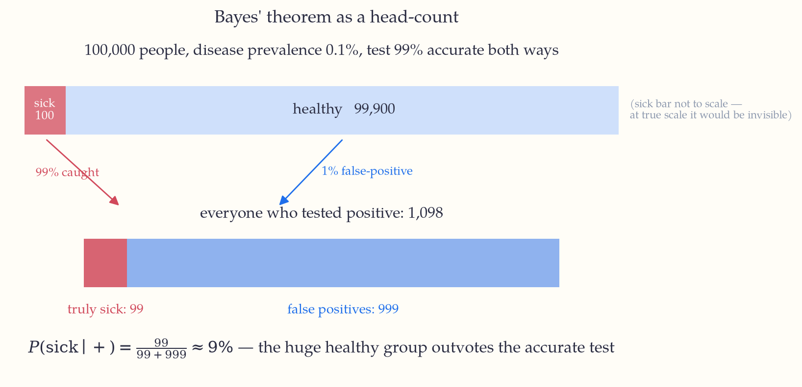
Key idea. Bayes’ theorem is why medical test results surprise people. A 99%-accurate test for a disease afflicting 1 in 1000: among 100,000 people, ~100 have it (99 test positive) while ~99,900 don’t (about 999 false positives). A positive result means only \frac{99}{99+999} \approx 9\% chance of disease. The rarity of the condition overwhelms the accuracy of the test.

Worked example (independence in practice). A server has two independent backup power units, each failing in a given year with probability 0.05. P(\text{both fail}) = 0.05^2 = 0.0025 — redundancy multiplies small numbers into tiny ones. But if both units share a fuel supply, the failures are not independent, and the naive multiplication dangerously flatters the system. Checking independence before multiplying is half of applied probability.

Random variables and distributions#

A random variable attaches a number to each outcome; its expected value E[X] = \sum x_i p_i is the long-run average, and its variance \mathrm{Var}(X) = E[(X-\mu)^2] measures spread (standard deviation \sigma = \sqrt{\mathrm{Var}}).

The binomial distribution counts successes in n independent yes/no trials with success probability p: \begin{aligned}P(X = k) = \binom{n}{k} p^k (1-p)^{n-k}, \\ E[X] = np, \\ \mathrm{Var}(X) = np(1-p).\end{aligned}

And looming behind nearly all of statistics stands the normal distribution, the bell curve f(x) = \frac{1}{\sigma\sqrt{2\pi}} e^{-(x-\mu)^2/2\sigma^2}:

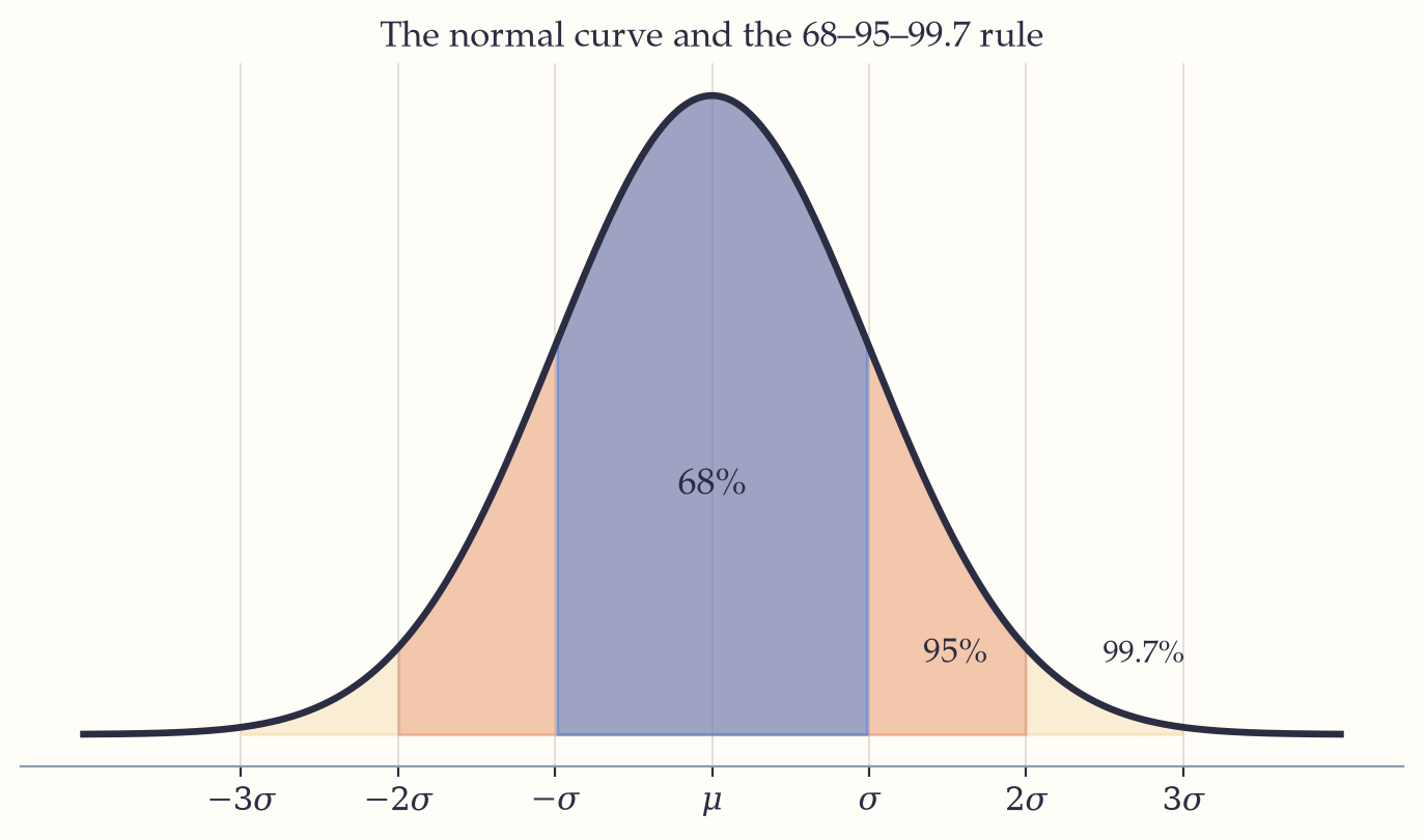
About 68% of its mass lies within one standard deviation of the mean, 95% within two, 99.7% within three. Why the bell curve appears everywhere is a genuine theorem — the Central Limit Theorem — kept for Chapter 20.

In the wild. Spam filters were the first mass-market Bayes’ theorem (word frequencies update the odds a message is spam); the same “naive Bayes” classifier is still a strong baseline in ML. A/B tests deciding which button ships are hypothesis tests (Chapter 20). And every language model is, at bottom, a machine for conditional probability: P(\text{next word} \mid \text{words so far}).

If you keep one thing from this chapter: Count by multiplying independent choices, divide out order when it doesn’t matter, and let Bayes’ theorem reweight every test result by its base rate.