Differential Equations
Equations whose unknowns are functions#
A differential equation relates a function to its derivatives: it describes not a quantity but a law of change, and solving it means recovering the quantity from the law. This is the mathematics in which physics, biology, epidemiology, and finance are actually written.
The picture to hold: a first-order equation y' = f(x, y) assigns a tiny slope to every point of the plane — a slope field — and a solution is a curve that flows along the field:
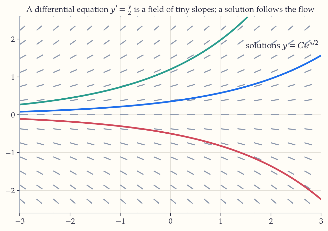
Through each starting point (initial condition) threads exactly one solution curve: the same law of change, launched from different beginnings.
The solvable classics#
Separable equations — get each variable on its own side and integrate: \begin{gathered}\frac{dy}{dx} \\ = ky \\ \Rightarrow \int\frac{dy}{y} \\ = \int k\,dx \\ \Rightarrow \ln|y| \\ = kx + C \\ \Rightarrow y \\ = Ae^{kx}.\end{gathered} This single computation is exponential growth and radioactive decay: “rate proportional to amount” forces the exponential. Newton’s cooling, logistic population growth, and simple epidemics are all separable.
First-order linear equations y' + P(x)y = Q(x) — multiply through by the integrating factor \mu = e^{\int P\,dx}. Why that strange multiplier? Because it is engineered so that \mu' = P\mu (differentiate e^{\int P\,dx} by the chain rule to see it), and then the left side collapses into a single derivative by the product rule: \mu y' + \mu P y = \mu y' + \mu' y = (\mu y)'. A full run:
Solve y' + 2y = e^{-x}.
- Here P(x) = 2, so the factor is \mu = e^{\int 2\,dx} = e^{2x}
\begin{aligned}&\text{2. Multiply the whole equation by } \mu: && e^{2x}y' + 2e^{2x}y = e^{2x}e^{-x} = e^{x}\end{aligned}
Recognize the left side as one derivative: \big(e^{2x}y\big)' = e^{x} \quad (product rule, run backwards)
Integrate both sides: e^{2x}y = \int e^x dx = e^x + C
\begin{aligned}&\text{5. Divide by } e^{2x}: && y = e^{-x} + Ce^{-2x}.\end{aligned}
Verify: y' = -e^{-x} - 2Ce^{-2x}, so y' + 2y = (-e^{-x} - 2Ce^{-2x}) + (2e^{-x} + 2Ce^{-2x}) = e^{-x} ✓.
Second-order linear with constant coefficients ay'' + by' + cy = 0 — guess y = e^{rx} and the ODE becomes the characteristic equation ar^2 + br + c = 0. The discriminant of Chapter 4 returns with new meaning:
| Roots of ar^2+br+c=0 | General solution | Behavior |
|---|---|---|
| real distinct r_1, r_2 | c_1e^{r_1x} + c_2e^{r_2x} | growth/decay |
| real repeated r | (c_1 + c_2x)e^{rx} | critical case |
| complex \alpha \pm i\beta | e^{\alpha x}(c_1\cos\beta x + c_2\sin\beta x) | oscillation |
Complex roots produce sines and cosines — Euler’s formula again — which is why the mass on a spring, my'' + ky = 0, oscillates: its characteristic roots are \pm i\sqrt{k/m}, giving y = c_1\cos\omega t + c_2\sin\omega t with frequency \omega = \sqrt{k/m}. Add a damping term by' and the three rows of the table become the three fates of a shock absorber: overdamped, critically damped, underdamped.
For the non-homogeneous equation (= g(x) instead of 0), the full solution is particular + homogeneous — structurally identical to linear systems in Chapter 16, because differentiation is a linear map and this is its rank–nullity story.
Worked example (the SIR epidemic sketch). Divide a population into Susceptible, Infected, Recovered fractions. The simplest model says S' = -\beta SI, I' = \beta SI - \gamma I, R' = \gamma I: infections need contact (SI product), recovery drains I at rate \gamma. One consequence read directly from the equations: the epidemic grows exactly while \beta S > \gamma, i.e. while S > \gamma/\beta — the herd-immunity threshold, visible without solving anything. Reading qualitative behavior off an ODE is often worth more than a formula.
In the wild. ODEs are the native language of dynamic systems: circuits (RLC), chemistry (reaction rates), pharmacology (drug concentration), rockets, climate, predator–prey ecology. Numerically “solving” them (Euler, Runge–Kutta) powers every physics engine and simulation — and, in a lovely convergence, the residual networks and diffusion models of modern AI are discretized ODEs.
If you keep one thing from this chapter: A differential equation is a law of change; solving it recovers the quantity from the law, and through each initial condition flows exactly one future.
Exercises 18
- Solve y' = \dfrac{x}{y} with y(0) = 2; describe the solution curves geometrically.
- Solve y' + y = x by integrating factor. (You will need integration by parts from Chapter 14 along the way.)
- Solve y'' - y' - 6y = 0 with y(0) = 1, y'(0) = 8.
- Solve y'' + 4y = 0 and identify the amplitude of the solution with y(0)=3, y'(0)=8.
- A cup of coffee at 90°C sits in a 20°C room and cools to 70°C in 5 minutes (Newton: rate proportional to temperature excess). When does it reach 40°C?