Probability, Information, and Learning
From scores to probabilities: softmax#
A classifier’s last layer emits raw scores (“logits”) — one real number per class. To act on them we need probabilities: non-negative, summing to 1. The softmax does the conversion with Chapter 5’s exponential:
\text{softmax}(z)_i = \frac{e^{z_i}}{\sum_j e^{z_j}}.
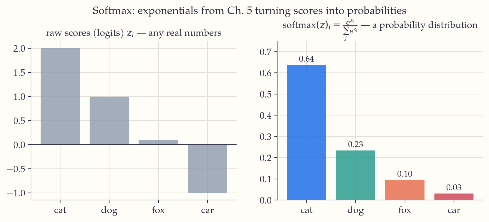
Exponentiating makes everything positive and amplifies differences (hence “softmax”: the biggest score takes most of the mass); dividing by the sum normalizes. Subtracting a constant from all logits changes nothing (the e^{c} cancels) — an identity of exponents that doubles as the standard numerical-stability trick. The sigmoid is softmax’s two-class special case.
Entropy and cross-entropy: counting surprise#
Information theory (Shannon, 1948) measures uncertainty in bits. The entropy of a distribution,
H(p) = -\sum_i p_i \log_2 p_i,
is the average surprise of its outcomes — maximal for a fair coin (1 bit), zero for a certainty. Two computations show the range:
\begin{aligned}H(\text{fair coin}) &= -\left(\tfrac12\log_2\tfrac12 + \tfrac12\log_2\tfrac12\right) = -(-\tfrac12-\tfrac12) = 1 \text{ bit}\end{aligned}
maximum for two outcomes
\begin{aligned}H(\text{90/10 coin}) &= -\left(0.9\log_2 0.9 + 0.1\log_2 0.1\right) \approx 0.47 \text{ bits}\end{aligned}
lopsided, so less surprising
\begin{aligned}H(\text{certain}) &= -\left(1\log_2 1\right) = 0 \text{ bits}\end{aligned}
no surprise at all
The biased coin still has two possible outcomes, yet carries under half the information of a fair one — because you can usually guess it. That is the precise sense in which a predictable message says less, and it is why compression works at all.
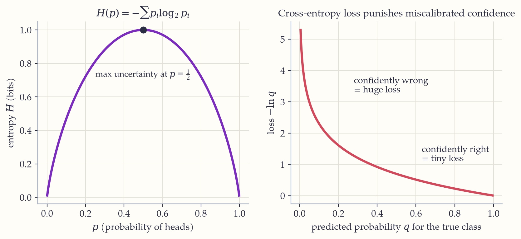
Cross-entropy H(p, q) = -\sum_i p_i \log q_i measures the surprise of using believed distribution q when truth is p. As a loss for classification, with p the one-hot true label, it collapses to -\log q_{\text{true}}: the model pays little for confident correct predictions and enormously for confident wrong ones (right panel of the figure). The gap D_{KL}(p\,\|\,q) = H(p,q) - H(p) — the Kullback–Leibler divergence — is the excess surprise, machine learning’s favorite measure of distance between distributions.
This is why classification uses cross-entropy rather than squared error: the loss is the logarithm of a probability, and logs turn products of probabilities into sums (Chapter 5) — which brings us to the principle underneath.
Maximum likelihood: why these losses and not others#
Where do loss functions come from? From probability run in reverse. Given data, the maximum likelihood principle says: choose the parameters under which the observed data was most probable,
\begin{gathered}\hat\theta \\ = \arg\max_\theta \; \prod_i P(\text{data}_i \mid \theta) \\ = \arg\max_\theta \; \sum_i \log P(\text{data}_i \mid \theta).\end{gathered}
Two beautiful specializations:
- Assume Gaussian noise around predictions, and maximizing likelihood becomes minimizing squared error — the normal density’s e^{-(y - \hat y)^2/2\sigma^2} turns, under \log, into the negative squared residual. Least squares is secretly a statement about bell curves.
- Assume the model outputs class probabilities, and maximizing likelihood becomes minimizing cross-entropy — the log of the probability assigned to the truth.
So the two great losses of ML are not conventions; they are theorems. Training a model is statistical estimation (Chapter 20), executed by gradient descent (Chapter 22), on matrix-shaped data (Chapter 21). The book’s three final threads braid into one cable.
Bayesian seasoning. Multiply the likelihood by a prior P(\theta) (Bayes’ theorem, Chapter 9) and maximize the posterior instead: the log-prior becomes an additive penalty on the loss. A Gaussian prior on weights yields exactly the L2 regularization (“weight decay”) term \lambda|\theta|^2 that practitioners add to keep weights small — regularization is a prior wearing overalls.
Generalization: the bias–variance bargain#
The goal is never to fit the training data — it is to predict the next example. A model too simple misses the signal (bias); a model too flexible memorizes the noise (variance):
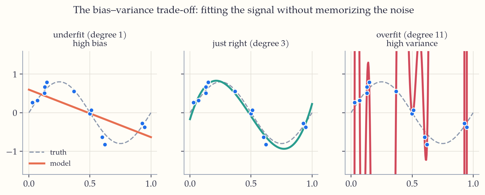
The degree-11 polynomial on the right passes through every point and would fail spectacularly on a new one — the mathematical portrait of overfitting. The defenses form the daily craft of ML: hold out test data to measure honestly (a Chapter-20 estimation problem), regularize to tame variance, and prefer the simplest model the evidence supports. The Central Limit Theorem makes one more appearance here: averaging many models (ensembling) shrinks variance like \frac{\sigma}{\sqrt{n}} — random forests are the CLT practiced on decision trees.
Where everything is used: the grand map#
Every chapter of this book is load-bearing somewhere in AI. A closing tour:
| You revised… | It powers… |
|---|---|
| Exponents & logs (Ch. 1, 5) | log-probabilities, softmax, log-loss, learning-rate schedules |
| Functions & composition (Ch. 3) | models as functions; deep nets as compositions |
| Quadratics (Ch. 4) | squared-error loss; convex bowls; Newton’s method |
| Trigonometry (Ch. 6) | positional encodings in transformers; Fourier features; signals |
| Sequences & series (Ch. 8) | discounted rewards in RL; convergence of training |
| Counting & probability (Ch. 9) | Bayes classifiers; language models as conditional probability |
| Vectors & dot products (Ch. 10) | embeddings; attention scores (QK^T) in transformers |
| Matrices (Ch. 12) | layers, batches, GPUs; adjacency matrices for graph nets |
| Derivatives & chain rule (Ch. 13) | backpropagation — all of it |
| Integrals (Ch. 14) | expectations; probability densities; diffusion models |
| Analysis (Ch. 15) | convergence guarantees; numerical stability |
| Linear algebra (Ch. 16) | PCA; SVD recommenders; spectral methods; PageRank |
| Multivariable calculus (Ch. 17) | gradients; Hessians; saddle points; Lagrange duality in SVMs |
| Differential equations (Ch. 18) | neural ODEs; diffusion models; physics-informed networks |
| Groups & fields (Ch. 19) | equivariant networks; cryptography guarding the models |
| Statistics (Ch. 20) | evaluation, confidence, A/B tests, maximum likelihood |
If one sentence should survive this book, let it be this: artificial intelligence is not new mathematics — it is the mathematics you already knew, finally given enough data and enough silicon to show what it could do.
If you keep one thing from this chapter: Softmax turns scores into probabilities, cross-entropy prices misplaced confidence, and maximum likelihood proves these losses are theorems, not conventions.
Exercises 23
- Compute softmax of z = (2, 0, -2) (three decimals), and verify the probabilities are unchanged if 10 is added to every logit.
- A model assigns the true class probability q = 0.9 on one example and q = 0.01 on another. Compute the cross-entropy loss of each. Which example dominates the gradient?
- Compute the entropy (in bits) of a die that shows 6 with probability \frac12 and each other face with probability \frac{1}{10}. Compare with a fair die.
- Show that maximizing \prod_i e^{-(y_i - w x_i)^2/2} over w is the same problem as least squares.
- You fit polynomials of degree 1–12 to 15 noisy points. Training error falls monotonically with degree, but test error falls then rises. Explain both facts using bias and variance.