Real Analysis: Calculus Grows Up
Why analysis exists#
School calculus runs on trust: limits “obviously” behave, curves “obviously” have areas. Analysis is what happened when 19th-century mathematicians (Cauchy, Weierstrass, Dedekind) stopped trusting and started proving — and discovered that the innocent-looking real line holds genuine monsters (functions continuous everywhere yet differentiable nowhere). The cure was precision.
Sequences, precisely#
A sequence (a_n) converges to L if the terms eventually stay inside any prescribed tolerance band around L:
\begin{gathered}\forall \varepsilon > 0,\; \exists N \in \mathbb{N}:\; n > N \implies |a_n \\ - L| < \varepsilon.\end{gathered}
Read it as a game: a skeptic names a tolerance \varepsilon (however tiny); you must produce a threshold N beyond which every term is within \varepsilon of L. If you can always win, the sequence converges.
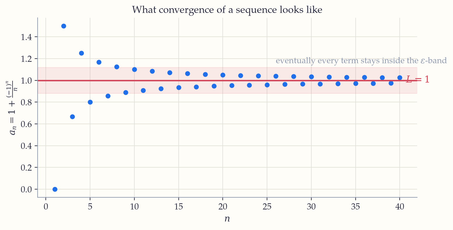
Worked proof. Claim: a_n = \frac{1}{n} \to 0. Given \varepsilon > 0, choose N > \frac{1}{\varepsilon}. Then n > N \implies |a_n - 0| = \frac{1}{n} < \frac{1}{N} < \varepsilon. \blacksquare Every convergence proof has this shape: from the demanded \varepsilon, reverse-engineer an N that works.
Two pillars hold up the whole theory, both equivalent to the completeness of \mathbb{R} (the “no gaps” promise of Chapter 1):
- Monotone Convergence Theorem: a bounded increasing sequence converges. (It has nowhere to go but up, and a ceiling — it must settle.)
- Bolzano–Weierstrass: every bounded sequence has a convergent subsequence.
Limits of functions and continuity#
The same game defines function limits — this is the famous \varepsilon–\delta definition:
\begin{gathered}\lim_{x \to a} f(x) \\ = L \\ \iff \forall \varepsilon > 0\; \exists \delta > 0:\; 0 < |x \\ - a| < \delta \implies |f(x) \\ - L| < \varepsilon.\end{gathered}
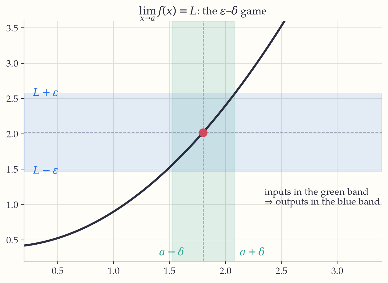
The picture makes it friendly: for every horizontal tolerance band (blue) around L, there must exist a vertical band (green) around a whose points all map into it. f is continuous at a when additionally L = f(a): no jump, no hole, no wild oscillation.
Continuity buys two theorems that sound obvious and are anything but:
- Intermediate Value Theorem: a continuous function on [a,b] takes every value between f(a) and f(b). (You cannot cross a river without getting wet.) This is why x^5 - x - 1 = 0 must have a root between 1 and 2: the polynomial is negative at 1, positive at 2.
- Extreme Value Theorem: a continuous function on a closed, bounded interval attains a maximum and minimum — the guarantee that makes optimization meaningful.
And the crown of differential calculus, the Mean Value Theorem: if f is continuous on [a,b] and differentiable inside, then somewhere the instantaneous slope equals the average slope: \begin{aligned}\exists\, c \in (a,b): \\ f'(c) = \frac{f(b) - f(a)}{b - a}.\end{aligned}
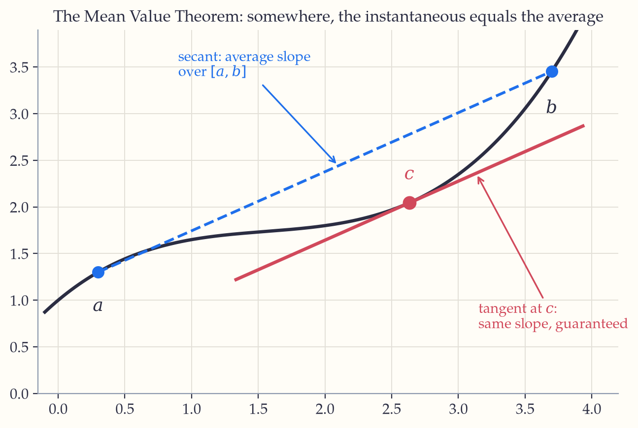
(If your average speed over an hour was 60 km/h, at some instant your speedometer read exactly 60.) Almost every hard fact about derivatives — “f' > 0 implies increasing”, error bounds for Taylor polynomials, L’Hôpital’s rule — is the MVT in costume.
Worked micro-proof, to see the MVT earn wages. Claim: if f'(x) = 0 for every x in an interval, then f is constant there. Take any two points a < b in the interval. The MVT hands us a c between them with f(b) - f(a) = f'(c)(b - a). But f'(c) = 0 by hypothesis, so f(b) = f(a) — any two values are equal, which is what “constant” means. \blacksquare Notice what the MVT did: it converted global information we wanted (“the function doesn’t change over an interval”) into local information we had (“the derivative is zero at each point”). That conversion, local \to global, is its entire career — and it is why antiderivatives are unique up to the constant +C: two of them differ by a function with zero derivative.
Infinite series, honestly#
An infinite series \sum a_n converges when its partial sums S_N = a_1 + \cdots + a_N converge as a sequence. The workhorse convergence tests:
| Test | Statement |
|---|---|
| Divergence test | if a_n \not\to 0, the series diverges (converse false!) |
| Comparison | 0 \le a_n \le b_n and \sum b_n converges \Rightarrow \sum a_n converges |
| Ratio test | \lim |a_{n+1}/a_n| = r: converges if r < 1, diverges if r > 1 |
| Integral test | \sum f(n) and \int_1^\infty f(x)dx converge or diverge together |
| Alternating series | alternating signs + terms decreasing to 0 \Rightarrow converges |
The ratio test is the one that earns its keep most often, because it turns a question about infinitely many terms into a single limit. On \sum \frac{n!}{n^n}, which no comparison handles comfortably:
\begin{aligned}\frac{a_{n+1}}{a_n} &= \frac{(n+1)!}{(n+1)^{n+1}} \cdot \frac{n^n}{n!}\end{aligned}
divide the term by its predecessor
\begin{aligned}&= \frac{(n+1)\,n^n}{(n+1)^{n+1}} = \frac{n^n}{(n+1)^n} \\ &\quad \text{the factorials collapse — one factor of } (n+1) \\ &= \left(\frac{n}{n+1}\right)^{n} = \left(1 + \tfrac1n\right)^{-n} \longrightarrow e^{-1}\end{aligned}
Chapter 5’s limit, arriving where it is needed
Since e^{-1} \approx 0.368 < 1, the series converges. Note what happened: a fearsome-looking sum was settled by a limit you already knew. That is the pattern of analysis — the hard object is tamed by a familiar one.
The boundary cases are the famous ones: the harmonic series \sum \frac{1}{n} diverges (even though its terms vanish!), while \sum \frac{1}{n^2} = \frac{\pi^2}{6} converges. In general \sum \frac{1}{n^p} converges exactly when p > 1.
Taylor series rebuild functions from their derivatives at a single point:
\begin{aligned}f(x) = \sum_{n=0}^{\infty} \frac{f^{(n)}(a)}{n!}(x - a)^n,\end{aligned}
e.g.
\begin{aligned}\sin x = x - \frac{x^3}{3!} + \frac{x^5}{5!} - \cdots\end{aligned}
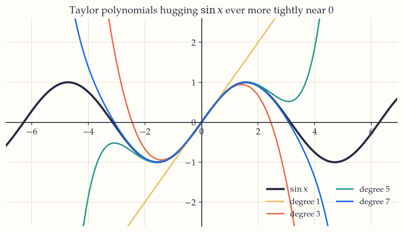
Each added term extends the polynomial’s embrace of the true curve. This is how calculators actually compute \sin, e^x, and \ln — and how Euler’s formula e^{i\theta} = \cos\theta + i\sin\theta is proved: substitute i\theta into the series for e^x and watch it split into the series for cosine and sine.
In the wild. Analysis is the safety engineering of computation. Floating-point arithmetic violates the field axioms subtly (addition isn’t associative in floating point!), and numerical analysis — the study of when algorithms converge and how errors grow — is applied real analysis. When a training run diverges or a physics simulation explodes, the diagnosis is written in this chapter’s language: an unstable iteration is a sequence that fails to converge.
If you keep one thing from this chapter: Analysis replaces trust with the \varepsilon–\delta game, and the completeness of \mathbb{R} — no gaps — underwrites every convergence theorem in calculus.
Exercises 15
- Prove from the definition that \dfrac{2n+1}{n+3} \to 2.
- Show the sequence a_1 = \sqrt2, a_{n+1} = \sqrt{2 + a_n} is increasing and bounded above by 2; conclude it converges and find its limit.
- Decide convergence: (a) \sum \dfrac{n}{n^2+1} (b) \sum \dfrac{n!}{n^n} (c) \sum \dfrac{(-1)^n}{\sqrt n}. (Part (b) is worked in this chapter — do it from memory first.)
- Use the IVT to show \cos x = x has a solution in (0, 1).
- Write the Taylor series of \ln(1+x) about 0 and state where it converges.