Multivariable Calculus

Functions of several variables#

A function f(x, y) assigns a height to each point of the plane — its graph is a surface, and its level curves (contour lines, as on a hiking map) trace where the height is constant.

Derivatives now come in directions. The partial derivative \frac{\partial f}{\partial x} differentiates in the x-direction, holding y frozen (and vice versa). For f(x,y) = x^2 + \tfrac{1}{2}y^2: \ \frac{\partial f}{\partial x} = 2x, \ \frac{\partial f}{\partial y} = y.

Bundle the partials into a vector and you get the object that organizes the whole subject — the gradient:

\nabla f = \left(\frac{\partial f}{\partial x},\; \frac{\partial f}{\partial y}\right).

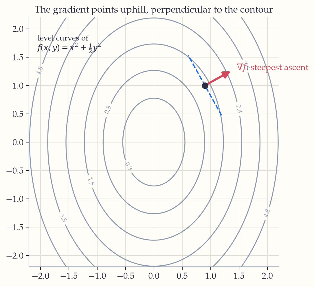
Key idea. The gradient points in the direction of steepest ascent, its length is the steepness, and it is always perpendicular to the level curves (along a contour the height doesn’t change, so all the change is crosswise). Gradient descent — walking against \nabla f — is how machine learning trains virtually every model.

The rate of change in an arbitrary unit direction \hat u is the directional derivative D_{\hat u}f = \nabla f \cdot \hat u, maximized when \hat u aligns with the gradient — the dot product of Chapter 10 earning its keep.

Optimization mirrors the one-variable story: interior extrema require \nabla f = 0; the second-derivative test now examines the Hessian determinant D = f_{xx}f_{yy} - f_{xy}^2 (D>0: max or min by sign of f_{xx}; D < 0: a saddle point — a mountain pass, minimum along one direction, maximum along another). The saddle is the genuinely new phenomenon here, so it is worth meeting one. Classify the critical points of f(x,y) = x^3 - 3xy + y^3:

\begin{aligned}f_x = 3x^2 - 3y = 0,\quad f_y = 3y^2 - 3x = 0\end{aligned}

set both partials to zero

\begin{aligned}\Rightarrow\ y = x^2 \text{ and } x = y^2 \;\Rightarrow\; x = x^4\end{aligned}

substitute one into the other

\begin{aligned}\Rightarrow\ x = 0 \text{ or } x = 1 \;\Rightarrow\; (0,0) \text{ and } (1,1)\end{aligned}

two critical points

\begin{aligned}f_{xx} = 6x,\quad f_{yy} = 6y,\quad f_{xy} = -3\end{aligned}

second partials, for the test

\begin{aligned}D = 36xy - 9:\qquad D(0,0) = -9 < 0 && \Rightarrow\ saddle \\ D(1,1) = 27 > 0,\ f_{xx}(1,1) = 6 > 0 && \Rightarrow\ local minimum\end{aligned}

At (0,0) the surface rises in one direction and falls in another — a mountain pass. This is not an exotic case: in the high-dimensional loss landscapes of Chapter 22, saddle points vastly outnumber genuine minima, and escaping them is much of what training a network actually involves.

Constrained problems (“optimize f on the curve g = c”) are handled by Lagrange multipliers. The insight is geometric: walking along the constraint curve, you are still improving f whenever the curve cuts across f’s level curves; the best point is where the constraint runs parallel to a level curve — where they kiss. Parallel curves have parallel normals, and normals are gradients (the contour figure earlier in this chapter), so at the optimum \nabla f = \lambda \nabla g for some multiplier \lambda. Worked in full:

Maximize f(x,y) = xy subject to g(x,y) = x + y = 10.

1. Compute both gradients: \nabla f = (y,\ x), \qquad \nabla g = (1,\ 1)

2. Set \nabla f = \lambda \nabla g — two equations: y = \lambda, \qquad x = \lambda

3. So x = y. Feed this into the constraint: x + x = 10 \;\Rightarrow\; x = y = 5

4. Evaluate: f(5,5) = 25.

Sanity check by intrusion: nearby constraint points (4,6) and (6,4) give f = 24 < 25 ✓. (This tiny problem is the ancient isoperimetric fact that among rectangles of fixed perimeter, the square encloses the most area.)

Multiple integrals#

A double integral \iint_R f(x,y)\,dA adds up f over a 2-D region — volume under a surface, total mass from a density, probability from a joint density. Compute it as an iterated integral, one variable at a time (Fubini’s theorem):

\begin{gathered}\int_0^1 \int_0^2 (x + y^2)\,dy\,dx \\ = \int_0^1 \left[xy + \frac{y^3}{3}\right]_{y=0}^{2} dx \\ = \int_0^1 \left(2x + \frac{8}{3}\right)dx \\ = 1 + \frac{8}{3} \\ = \frac{11}{3}.\end{gathered}

Round regions beg for polar coordinates x = r\cos\theta, y = r\sin\theta, with the crucial area element dA = r\,dr\,d\theta (the r is the Jacobian — small polar rectangles far from the origin are bigger). The most beautiful payoff: the Gaussian integral, impossible in one dimension, surrenders in two —

\left(\int_{-\infty}^{\infty} e^{-x^2}dx\right)^2 = \iint e^{-(x^2+y^2)}dA = \int_0^{2\pi}\!\!\int_0^\infty e^{-r^2} r\,dr\,d\theta = \pi \;\Longrightarrow\; \int_{-\infty}^{\infty} e^{-x^2}dx = \sqrt{\pi},

which is precisely why the normal distribution carries its factor of \sqrt{2\pi}.

In the wild. Multivariable calculus is the mathematics of many knobs. A modern neural network is a function of millions of variables, and its training loop — compute \nabla L, step against it — is this chapter’s gradient, iterated (Chapter 22). Lagrange multipliers reappear in economics (constrained utility), in SVMs (the “support vectors” are multiplier conditions), and in physics (constrained motion). The Hessian’s saddle points turn out to dominate high-dimensional loss landscapes.

If you keep one thing from this chapter: The gradient points straight uphill, perpendicular to the level curves. All optimization in many dimensions — including machine learning — either follows it or fights it.