Linear Algebra: The Study of Flat Things

Vector spaces: the abstraction that pays#

Chapter 10’s arrows and Chapter 12’s matrices were previews. The mature subject begins by asking: what do arrows, polynomials, matrices, and solutions of linear differential equations have in common? Answer: you can add them and scale them, subject to the natural laws. Any such system is a vector space, and one theory now serves them all — the great economy of abstraction.

The central vocabulary:

• A linear combination of v_1, \dots, v_k is c_1v_1 + \cdots + c_kv_k.
• Their span is the set of all linear combinations — the flat sheet they generate.
• They are linearly independent if no one of them is a combination of the others (equivalently: c_1v_1 + \cdots + c_kv_k = 0 only when all c_i = 0). Independence means no redundancy.
• A basis is an independent spanning set: a minimal coordinate system. Every basis of a space has the same size — its dimension.

In \mathbb{R}^3, the standard basis is \hat i, \hat j, \hat k; but the space of polynomials of degree \le 2 is also 3-dimensional, with basis \{1, x, x^2\}. Same theory, different costumes.

Linear maps, rank, and the conservation of dimension#

A linear map T respects the structure: T(u + v) = T(u) + T(v) and T(cv) = cT(v). Once you fix bases, every linear map is a matrix. Two subspaces measure what a map does:

• the kernel (null space): everything crushed to zero;
• the image (column space): everything reachable; its dimension is the rank.

They balance perfectly — the Rank–Nullity Theorem: \dim(\ker T) + \operatorname{rank} T = \dim(\text{domain}). Dimension is never created, only preserved or crushed. A system A\vec x = \vec b is solvable exactly when \vec b lies in the image; the solution set, when nonempty, is one particular solution plus the whole kernel — the same “particular + homogeneous” structure that will reappear in differential equations.

Eigenvalues: a matrix’s true personality#

A matrix shuffles most vectors’ directions. Its eigenvectors are the exceptions — directions it merely stretches:

\begin{aligned}A\vec v = \lambda \vec v, \\ \vec v \ne 0.\end{aligned}

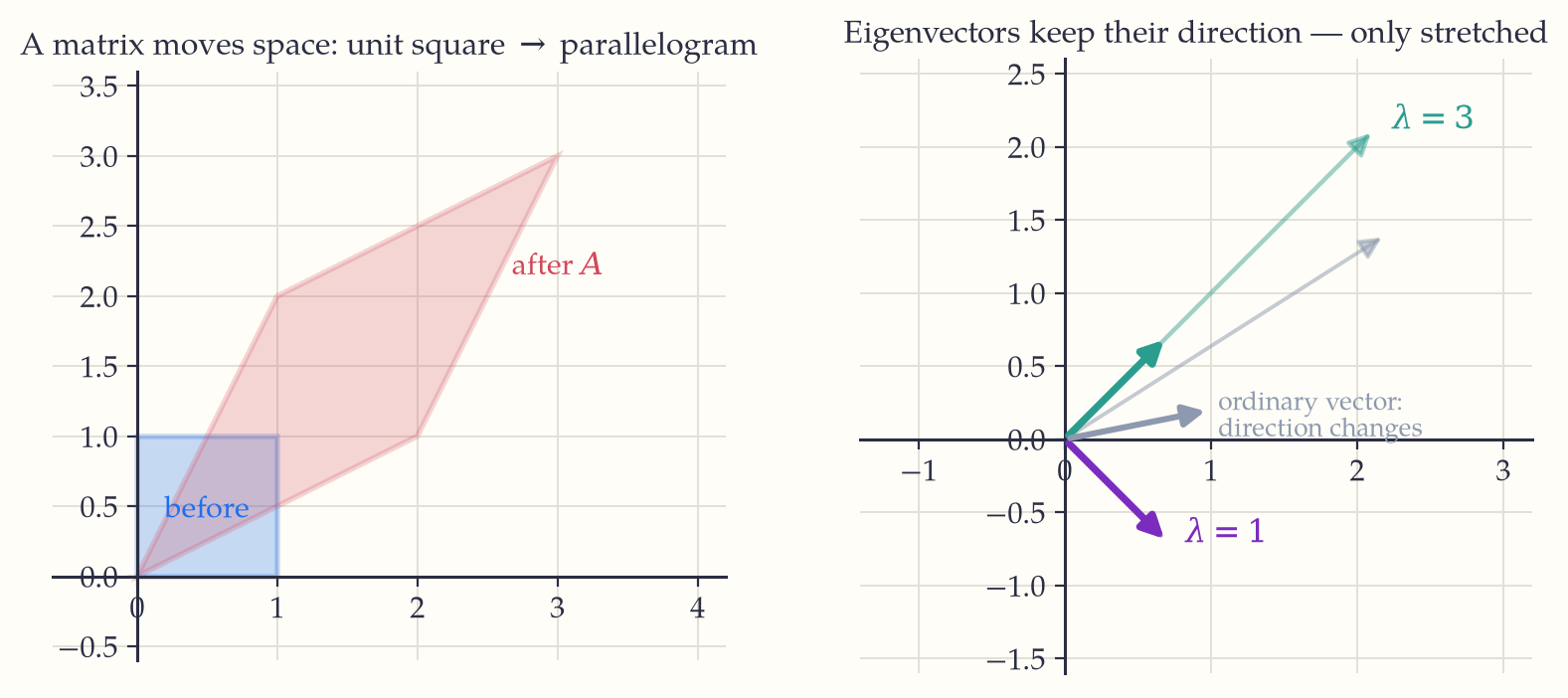
Why does \det(A - \lambda I) = 0 find them? Rearrange the definition: A\vec v = \lambda\vec v means (A - \lambda I)\vec v = \vec 0 with \vec v \ne 0 — the matrix A - \lambda I crushes a nonzero vector to zero, and Chapter 12 told us exactly when a matrix destroys information: when its determinant vanishes. The full procedure, narrated on A = \begin{pmatrix}2&1\\1&2\end{pmatrix}:

\begin{aligned}&\text{1. Form } A - \lambda I \text{ (subtract down the diagonal):} && \begin{pmatrix} 2-\lambda & 1 \\ 1 & 2-\lambda \end{pmatrix}\end{aligned}

2. Set its determinant to zero: (2-\lambda)(2-\lambda) - (1)(1) = 0

3. Solve the resulting polynomial: (2-\lambda)^2 = 1 \;\Rightarrow\; 2 - \lambda = \pm 1 \;\Rightarrow\; \lambda = 1,\ 3

\begin{aligned}&\text{4. For each } \lambda\text{, solve } (A - \lambda I)\vec v = \vec 0. && \\ &\phantom{4.}\ \lambda = 3:\; \begin{pmatrix} -1 & 1 \\ 1 & -1\end{pmatrix}\!\begin{pmatrix} v_1 \\ v_2\end{pmatrix} = \vec 0 \\ &\quad \text{row 1: } -v_1 + v_2 = 0 \Rightarrow v_2 = v_1 \\ &\phantom{4.}\ \text{so any multiple of } (1, 1) \text{ works.}\end{aligned}

(row 2 says the same)

\begin{aligned}&\phantom{4.}\ \lambda = 1:\; \begin{pmatrix} 1 & 1 \\ 1 & 1\end{pmatrix}\!\begin{pmatrix} v_1 \\ v_2\end{pmatrix} = \vec 0 && v_1 + v_2 = 0 \;\Rightarrow\; \text{eigenvector } (1, -1).\end{aligned}

Check (never skip it): A\begin{pmatrix}1\\1\end{pmatrix} = \begin{pmatrix}3\\3\end{pmatrix} = 3\begin{pmatrix}1\\1\end{pmatrix} ✓. These are exactly the green and purple arrows in the figure. Note the redundancy in step 4 — the two rows of (A - \lambda I) gave the same equation. That is not an accident but a confirmation: the matrix is singular at an eigenvalue, so its rows must be dependent; if your rows give conflicting equations, the \lambda was wrong.

When a matrix has a full basis of eigenvectors, it diagonalizes: A = PDP^{-1} with D diagonal. In the eigenbasis, the fearsome machine is revealed as independent stretches along independent axes — and hard problems collapse: A^{100} = PD^{100}P^{-1}, computed in a heartbeat since D^{100} just raises diagonal entries to the 100th power. This one trick powers population models, Markov chains, Google’s PageRank, principal component analysis, and the solution of linear ODE systems.

Key idea. Symmetric matrices (A = A^T) are the aristocracy: the Spectral Theorem guarantees their eigenvalues are real and their eigenvectors can be chosen mutually perpendicular. Nature’s symmetric matrices — covariance, inertia, quadratic forms — always admit clean perpendicular axes.

In the wild. Google’s original PageRank is an eigenvector: the importance vector of the web’s link matrix. PCA (Chapter 21) diagonalizes a covariance matrix to find the directions data actually varies in. Recommender systems factor the user–item matrix (SVD, diagonalization’s rectangular cousin); vibration engineers find a bridge’s resonant modes as eigenvectors; quantum energy levels are eigenvalues. Whenever a system has “natural modes,” eigentheory names them.

If you keep one thing from this chapter: Linear algebra measures flat structure: basis and dimension say how big, rank–nullity says what survives a map, and eigenvectors are the directions a map cannot turn.