Probability Theory and Statistics

Probability, refounded#

Chapter 9 counted equally likely outcomes; the mature theory (Kolmogorov, 1933) starts instead from axioms. A probability measure P assigns to events numbers in [0,1], with P(\text{everything}) = 1 and additivity over disjoint events — and the entire subject unfolds deductively from there, now able to handle infinite and continuous situations where “counting outcomes” is meaningless.

Continuous random variables have a density f(x): probabilities are areas, computed by the integrals of Chapter 14:

\begin{aligned}P(a \le X \le b) = \int_a^b f(x)\,dx, \\ E[X] = \int_{-\infty}^{\infty} x f(x)\,dx.\end{aligned}

The uniform, exponential (waiting times), and normal distributions are the repertory company. For the normal, the \sqrt{2\pi} in its formula is exactly the Gaussian integral we conquered with polar coordinates in Chapter 17 — the book’s threads knotting together.

The two great limit theorems#

Law of Large Numbers. The average of n independent copies of X converges to E[X] as n \to \infty. Casinos and insurance companies are machines built on this theorem: individual outcomes are unknowable, averages are destiny.

Central Limit Theorem. Far deeper: the distribution of the sum (or mean) of many independent variables approaches the normal distribution — almost regardless of the distribution you started with:

\frac{\bar X_n - \mu}{\sigma/\sqrt{n}} \;\longrightarrow\; N(0, 1).

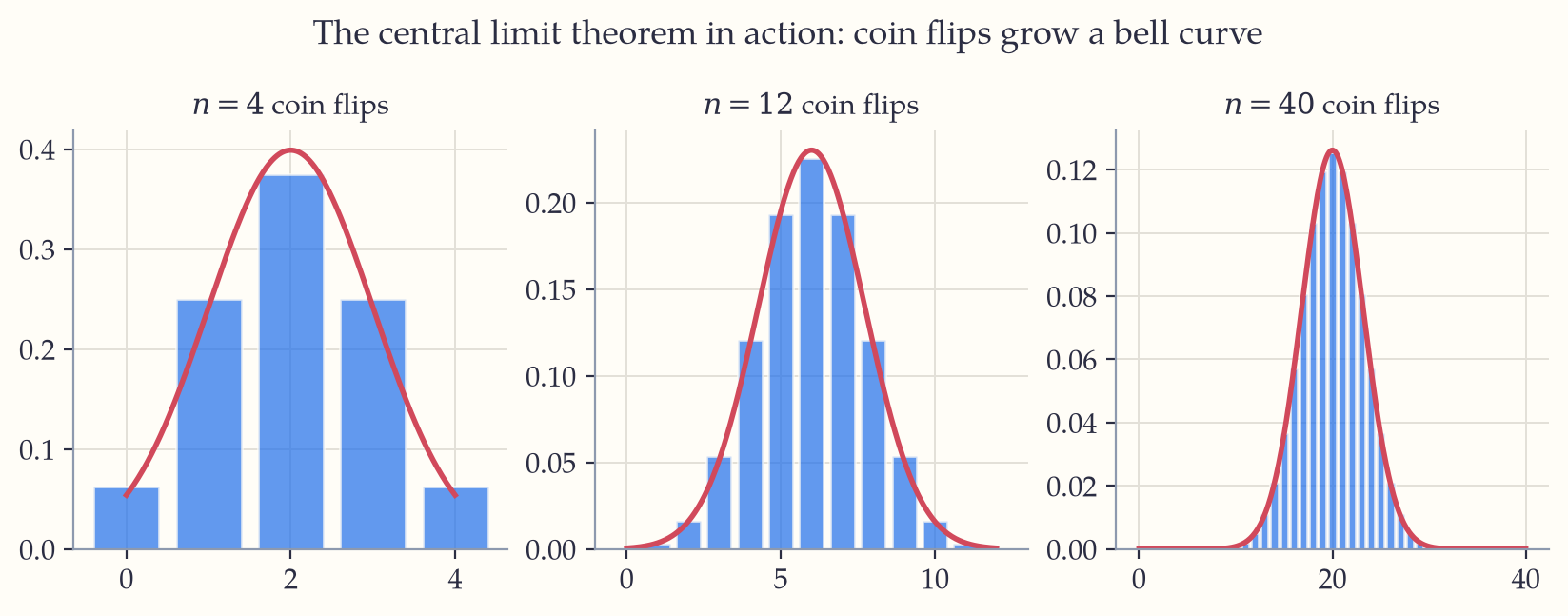
Coin flips are as non-normal as randomness gets (two spikes!), yet their sums grow a flawless bell. This is why the normal curve haunts nature: heights, measurement errors, noise — anything that is the sum of many small independent influences must be approximately normal. The bell curve is not an assumption about the world; it is a theorem about addition.

Statistics: reasoning backwards#

Probability reasons forward (model \to predicted data); statistics reasons backward (observed data \to inferred model). The core toolkit:

Estimation. The sample mean \bar x estimates \mu; the sample variance s^2 = \frac{1}{n-1}\sum(x_i - \bar x)^2 estimates \sigma^2 (the n-1 corrects the bias from measuring spread around \bar x rather than the true \mu). By the CLT, \bar x is approximately normal with standard error \sigma/\sqrt n — so a 95% confidence interval for \mu is

\bar x \pm 1.96\,\frac{s}{\sqrt n},

the 1.96 being the point that traps 95% of the standard normal (the “\pm 2\sigma” of the 68–95–99.7 rule, sharpened). Worked on real numbers: 64 measurements give \bar x = 12.4 with s = 3.2.

\begin{aligned}\text{standard error} &= \frac{s}{\sqrt n} = \frac{3.2}{\sqrt{64}} = \frac{3.2}{8} = 0.4 \\ &\quad \text{how much } \bar x \text{ itself wobbles} \\ \text{margin} &= 1.96 \times 0.4 = 0.784\end{aligned}

95% of that wobble

\begin{aligned}\text{interval} &= 12.4 \pm 0.78 = (11.62,\ 13.18).\end{aligned}

the honest answer, with its uncertainty

Read it correctly, because almost everyone does not: this does not say there is a 95% chance \mu lies in (11.62, 13.18). It says the procedure traps the true \mu in 95% of samples like this one. And note the \sqrt n: to halve the margin you need four times the data, not twice.

Hypothesis testing. Assume a skeptical null hypothesis H_0 (the drug does nothing; the coin is fair), compute how surprising the observed data would be under it (the p-value), and reject H_0 if the surprise is extreme (conventionally p < 0.05). A coin giving 60 heads in 100 flips: under fairness, \bar X has standard error 0.05, so 0.60 is z = 2 standard errors out — p \approx 0.046 — borderline suspicious. Ten times the data with the same proportion would be z = 6.3: overwhelming. Sample size is evidence.

Key idea. A p-value is not the probability the hypothesis is true — it is the probability of data this extreme if the null holds. Confusing the two is the most common statistical error in science. Bayes’ theorem (Chapter 9) is what converting between them actually requires.

Correlation and regression. The correlation coefficient r \in [-1, 1] measures linear association; least-squares regression fits the line minimizing squared vertical errors, with slope b = r\,\frac{s_y}{s_x}. And the eternal caution, which no refresher may omit: correlation is not causation — ice-cream sales and drownings rise together because of summer, not each other.

In the wild. Every ML model’s report card is statistics: train/test splits estimate generalization; confidence intervals qualify benchmark scores; A/B tests gate product launches. The bias-corrected s^2 and standard errors of this chapter are what “error bars” mean in every scientific paper. Chapter 23 completes the arc: training a model is statistical estimation — maximum likelihood — performed by the calculus of Chapter 22.