Quadratics and Polynomials

The parabola and its anatomy#

The quadratic y = ax^2 + bx + c graphs as a parabola: opening up if a > 0, down if a < 0, with its vertex at x = -\frac{b}{2a} and a mirror symmetry through that vertical line.

Completing the square is the key move of the whole chapter, so let us do it slowly. The idea: x^2 + px is almost the perfect square (x + \frac{p}{2})^2 = x^2 + px + \frac{p^2}{4} — it is only missing the constant \frac{p^2}{4}. So add and subtract that missing piece. A concrete run first:

\begin{aligned} x^2 + 6x + 1 &= \underbrace{x^2 + 6x + 9}_{\text{a perfect square}} - 9 + 1 \\ &\quad \text{add and subtract } \left(\tfrac{6}{2}\right)^2 = 9\\ &= (x + 3)^2 - 8 \\ &\quad \text{vertex form: lowest value } -8 \text{ at } x = -3. \end{aligned}

The name is literal — the algebra is a picture of tiling:

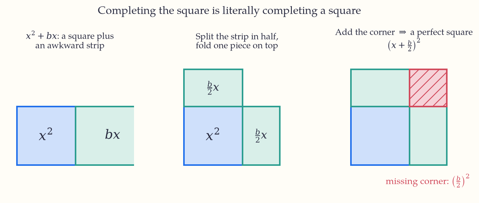
Now the same moves on the general quadratic ax^2 + bx + c = 0, one line at a time — this derivation is the quadratic formula, and once you have walked it, the formula stops being a magic spell:

\begin{aligned}ax^2 + bx + c &= 0 \\ &\quad \text{the general quadratic, } a \ne 0 \\ x^2 + \frac{b}{a}x + \frac{c}{a} &= 0 \\ &\quad \text{divide both sides by } a \\ x^2 + \frac{b}{a}x &= -\frac{c}{a}\end{aligned}

move the constant right

\begin{aligned}x^2 + \frac{b}{a}x + \left(\frac{b}{2a}\right)^{\!2} &= \left(\frac{b}{2a}\right)^{\!2} - \frac{c}{a}\end{aligned}

complete the square

\begin{aligned}\left(x + \frac{b}{2a}\right)^{\!2} &= \frac{b^2}{4a^2} - \frac{c}{a} = \frac{b^2 - 4ac}{4a^2}\end{aligned}

a perfect square; tidy the right

\begin{aligned}x + \frac{b}{2a} &= \pm\frac{\sqrt{b^2 - 4ac}}{2a}\end{aligned}

take square roots — both signs!

\begin{aligned}x &= \frac{-b \pm \sqrt{b^2 - 4ac}}{2a} \\ &\quad \text{subtract } \frac{b}{2a}.\end{aligned}

(A formula equivalent to this was known to Brahmagupta in 7th-century India, a millennium before symbolic notation existed — he stated it in words.) The same completed square, not set to zero, exposes the vertex of the graph:

ax^2 + bx + c = a\left(x + \frac{b}{2a}\right)^2 + \left(c - \frac{b^2}{4a}\right).

The quantity under the root, \Delta = b^2 - 4ac, is the discriminant — the fortune-teller of the quadratic:

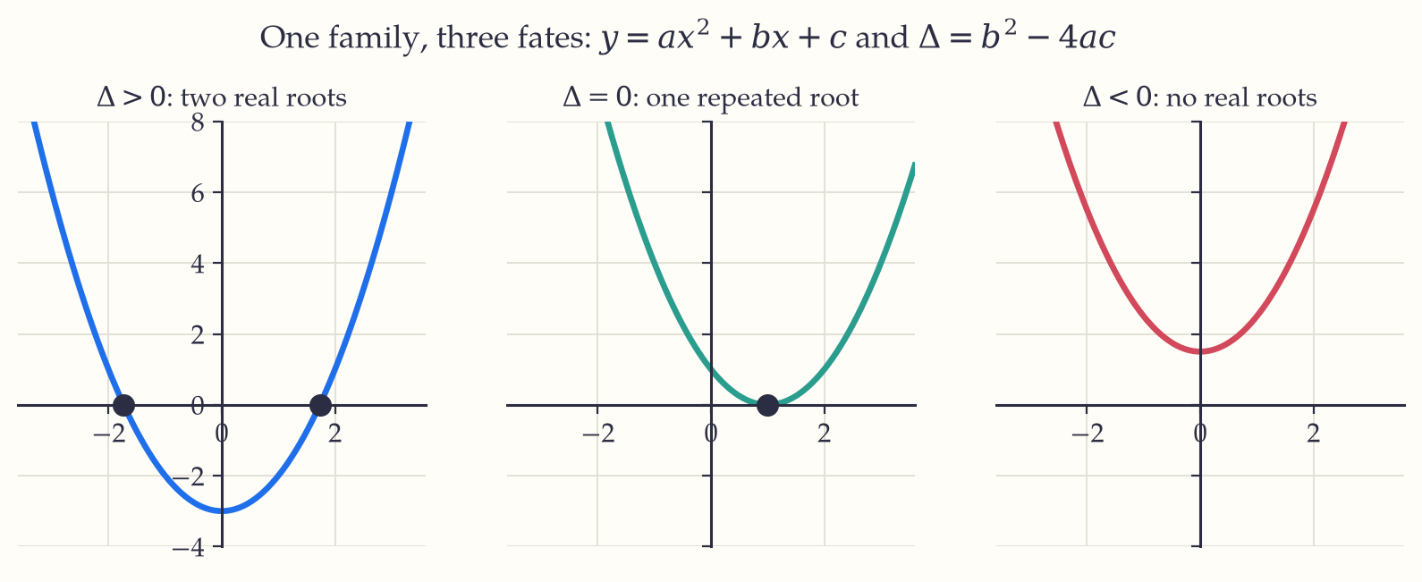
Key idea. \Delta > 0: two real roots (parabola crosses the axis twice). \Delta = 0: one repeated root (it kisses the axis). \Delta < 0: no real roots (it floats clear) — the roots have fled into the complex numbers, where Chapter 11 will find them.

Vieta’s formulas connect roots to coefficients without solving: if the roots are \alpha, \beta then \begin{aligned}\alpha + \beta = -\frac{b}{a}, \\ \alpha\beta = \frac{c}{a}.\end{aligned}

Polynomials in general#

A degree-n polynomial p(x) = a_nx^n + \dots + a_1x + a_0 has at most n real roots and at most n-1 turning points; for large |x| the leading term a_nx^n takes over completely and dictates the end behavior.

Two small theorems do most of the practical work:

• Remainder theorem: dividing p(x) by (x - a) leaves remainder p(a).
• Factor theorem: (x - a) divides p(x) exactly when p(a) = 0.

So to factor a cubic like p(x) = x^3 - 6x^2 + 11x - 6: test small candidates, find p(1) = 0, divide out (x-1) to get x^2 - 5x + 6, and finish with the quadratic: p(x) = (x-1)(x-2)(x-3).

The Fundamental Theorem of Algebra (proved only with complex numbers) says every degree-n polynomial has exactly n roots in \mathbb{C}, counted with multiplicity. Over the reals, complex roots hide in conjugate pairs — which is why odd-degree polynomials always have at least one real root.

If you keep one thing from this chapter: Completing the square is the master move: it exposes the vertex, derives the formula, and yields \Delta = b^2 - 4ac, the fortune-teller of the roots.