Vectors, Matrices, and Data

Data becomes geometry#

The founding move of machine learning is representational: everything becomes a vector. A house is (\text{area}, \text{bedrooms}, \text{age}, \dots) \in \mathbb{R}^{20}; a grayscale image is its pixel brightnesses, a point in \mathbb{R}^{784}; a customer is their purchase history. A dataset of n examples with d features is then an n \times d matrix X — one row per example, one column per feature. Chapter 10’s arrows and Chapter 12’s arrays were never just geometry homework; they are the file format of intelligence.

Once data is geometry, geometric questions become learning questions:

• How alike are two things? — a distance or an angle.
• What direction does the data vary in? — an eigenvector.
• What simple rule relates inputs to outputs? — a linear map.

Similarity: the dot product earns its living#

The workhorse measure of similarity is the cosine of the angle between two vectors — Chapter 10’s identity, read backwards:

\begin{gathered}\text{similarity}(\vec a, \vec b) \\ = \cos\theta \\ = \frac{\vec a \cdot \vec b}{|\vec a|\,|\vec b|} \in [-1, 1].\end{gathered}

A concrete pair makes the scale meaningful. Take \vec a = (3, 4) and \vec b = (4, 3):

\begin{aligned}\vec a \cdot \vec b &= (3)(4) + (4)(3) = 24\end{aligned}

the raw agreement

\begin{aligned}|\vec a| = |\vec b| &= \sqrt{9+16} = 5 \\ &\quad \text{both have length }5 \\ \cos\theta &= \frac{24}{5 \times 5} = 0.96 \\ &\quad \text{very similar — about }16°\text{ apart}\end{aligned}

Now double one of them, \vec b = (8,6): the dot product doubles to 48 and so does |\vec b|, leaving \cos\theta = 48/(5\times 10) = 0.96 — unchanged. That invariance is the whole reason cosine is used instead of the bare dot product: a document mentioning a word twice as often should not thereby be twice as relevant. Only direction carries the meaning.

Modern language AI rests on embeddings: words, sentences, and images are mapped to vectors in \mathbb{R}^{300}–\mathbb{R}^{10000} such that semantic similarity becomes geometric similarity.

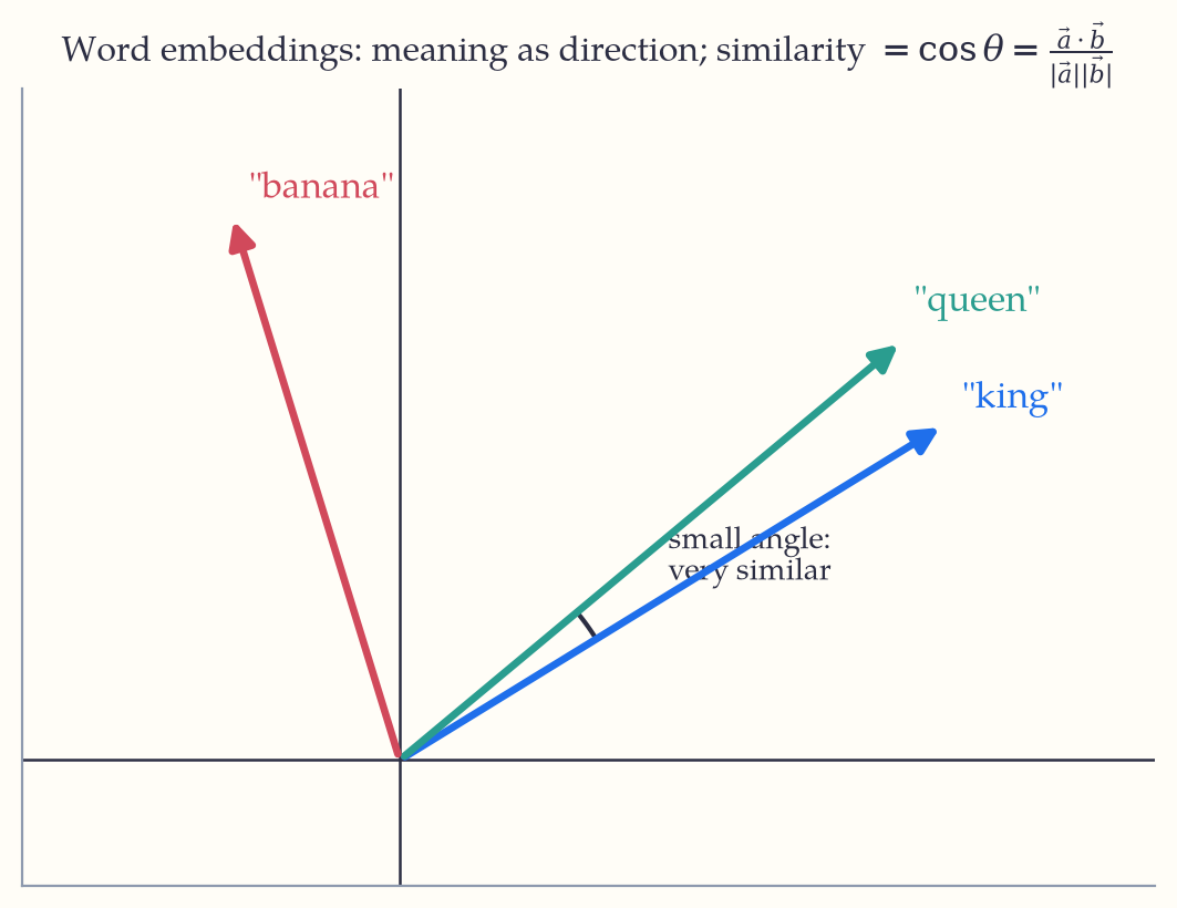
“King” and “queen” point in nearly the same direction; “banana” points elsewhere. Famously, embedding arithmetic captures analogy: \vec{v}_{\text{king}} - \vec{v}_{\text{man}} + \vec{v}_{\text{woman}} \approx \vec{v}_{\text{queen}} — the parallelogram rule of vector addition, discovering grammar. Every semantic search box, every “customers also bought,” every retrieval step inside a chatbot is a nearest-neighbor hunt under this cosine.

Worked example. Documents as (crude) word-count vectors over the vocabulary (math, movie, pizza): d_1 = (4, 0, 1), d_2 = (2, 0, 1), d_3 = (0, 5, 2). Then \cos(d_1, d_2) = \frac{8 + 0 + 1}{\sqrt{17}\sqrt{5}} = \frac{9}{9.22} \approx 0.98 (near-identical topics), while \cos(d_1, d_3) = \frac{2}{\sqrt{17}\sqrt{29}} \approx 0.09 (unrelated). A search engine ranking documents against your query performs exactly this computation, at scale.

Linear models: learning as solving X\vec w \approx \vec y#

The simplest learnable model predicts a target as a weighted sum of features:

\hat y = w_1 x_1 + w_2 x_2 + \cdots + w_d x_d + b = \vec w \cdot \vec x + b.

Learning means choosing the weights \vec w that best fit known examples — and “best” is Chapter 4’s quadratic idea: minimize the sum of squared errors L(\vec w) = |X\vec w - \vec y|^2.

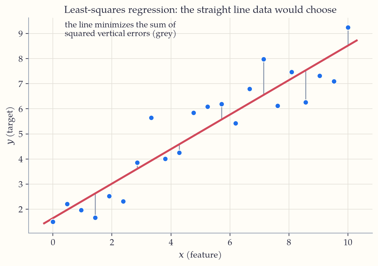
Because the loss is a quadratic bowl, calculus gives a closed-form answer — set the gradient to zero and solve the normal equations:

X^T X \, \vec w = X^T \vec y.

This is the one moment in machine learning where training is a single formula rather than an iteration. Two centuries old (Gauss used it to recover the lost asteroid Ceres in 1801), least squares is still the first model any practitioner fits — and the mental baseline against which deep learning is judged.

Layers are matrices; batches are matrix products#

A neural network layer computes \vec h = \sigma(W\vec x + \vec b): a matrix multiplication, a shift, a nonlinearity. Processing a whole batch of examples at once is the matrix product XW^T — which is why Chapter 12’s strange row-into-column rule, and hardware that performs it fast (GPUs, TPUs), together run the modern world. When you hear that a model has “7 billion parameters,” those parameters are, overwhelmingly, the entries of its weight matrices.

PCA: eigenvectors meet data#

Real datasets are redundant — features correlate, and the data cloud is effectively flat in most directions. Principal Component Analysis finds the flat structure: compute the covariance matrix C of the (centered) data, and diagonalize it. Being symmetric, C obeys the Spectral Theorem of Chapter 16: real eigenvalues, perpendicular eigenvectors.

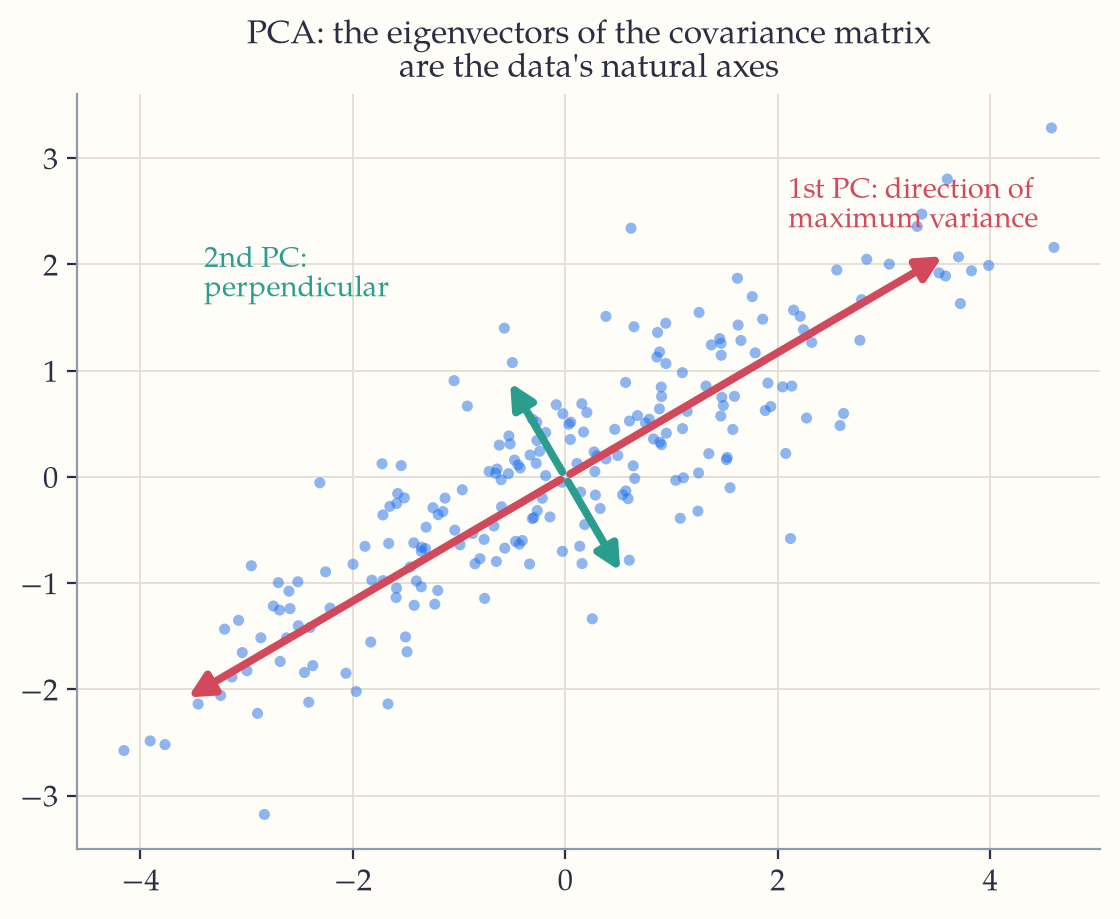
The eigenvector with the largest eigenvalue is the direction of maximum variance — the data’s own principal axis; the eigenvalues report how much variance each direction carries. Keeping only the top k eigenvectors compresses d-dimensional data to k dimensions while losing as little as possible — the optimal flat summary. PCA denoises sensor data, compresses images, visualizes high-dimensional datasets in 2-D, and preprocesses features across science; its rectangular generalization, the singular value decomposition (SVD), drove the Netflix-Prize era of recommender systems.

If you keep one thing from this chapter: Machine learning’s founding move: data becomes geometry. Vectors for things, cosine for similarity, matrix products for models, eigenvectors for the axes data truly varies along.