The Calculus of Learning

Loss: turning “wrong” into a number#

A model with parameters \theta makes predictions; a loss function L(\theta) scores how wrong they are on the training data — squared error for regression, cross-entropy (next chapter) for classification. The entire drama of training is then one sentence:

Learning is optimization. Find \theta minimizing L(\theta). Everything Chapter 13 said about minima — derivatives zero, second derivatives deciding — applies verbatim, except that \theta now has millions of coordinates, so we need Chapter 17: the gradient.

Gradient descent: rolling downhill in a million dimensions#

There is no formula for the minimum of a general loss, but there is a compass: \nabla L points uphill, so -\nabla L points down. Gradient descent simply walks:

\theta_{t+1} = \theta_t - \eta \, \nabla L(\theta_t),

where the learning rate \eta sets the stride.

Nothing here is mysterious once you run it by hand. Minimise L(w) = w^2 from w_0 = 4 with \eta = 0.25, using L'(w) = 2w:

\begin{aligned}w_1 &= 4 - 0.25(2\cdot 4) = 4 - 2 = 2\end{aligned}

step against the slope

\begin{aligned}w_2 &= 2 - 0.25(2\cdot 2) = 1\end{aligned}

the gradient shrank, so the step did too

\begin{aligned}w_3 &= 0.5,\quad w_4 = 0.25,\ \dots\end{aligned}

halving each time — a geometric sequence

Two things worth noticing, because both generalise to networks with billions of parameters. The steps get smaller by themselves as the slope flattens, so descent slows into a minimum rather than crashing through it. And the whole update is w \leftarrow (1 - 2\eta)w, a geometric sequence from Chapter 8: it converges exactly when |1-2\eta| < 1. Take \eta = 0.6 and the factor is -0.2 (still fine, but oscillating); take \eta = 1.2 and the factor is -1.4, so w grows without bound. That is the divergence every practitioner meets on their first badly-tuned run.

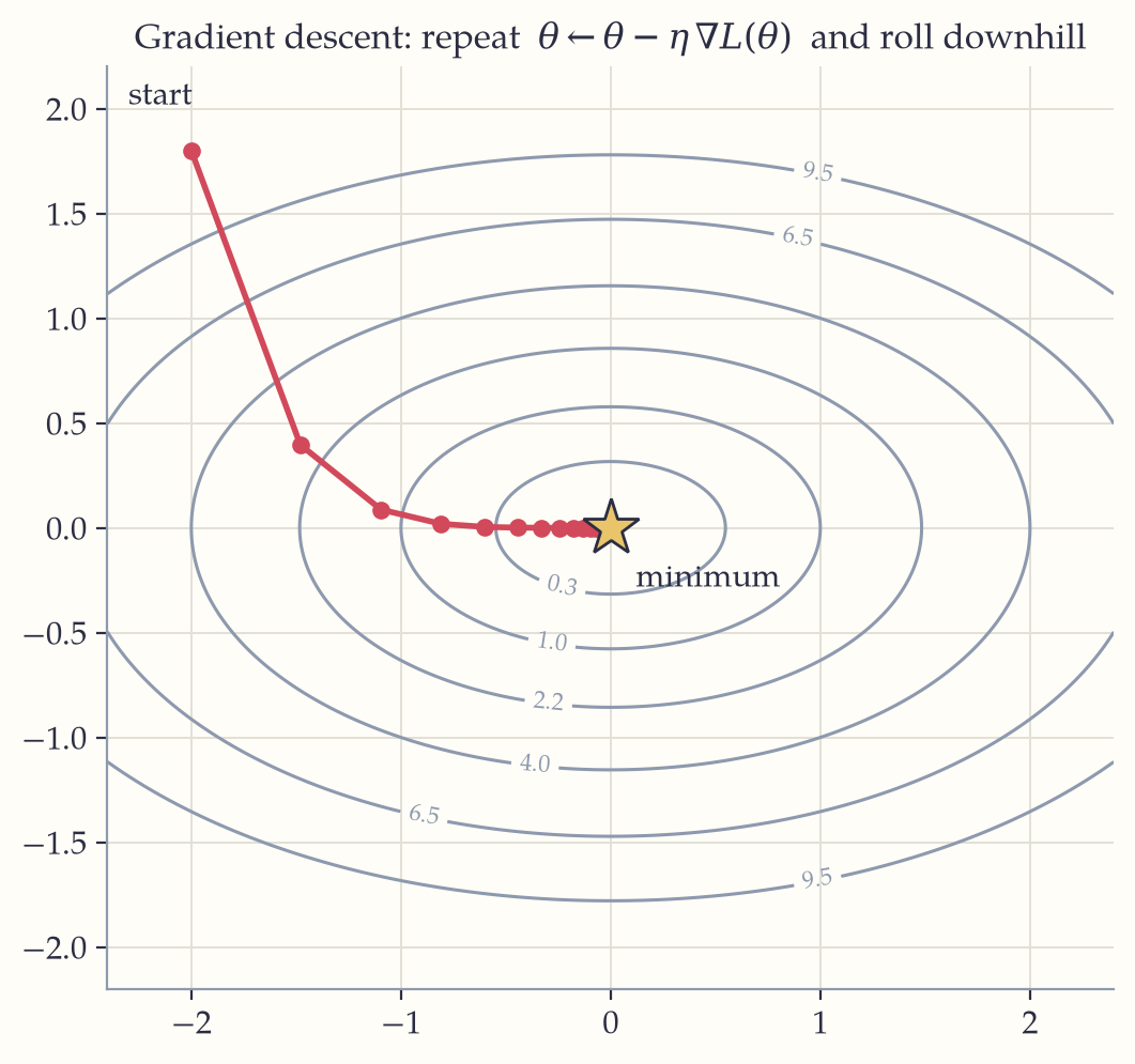
The picture shows the whole story, including its pathologies: on an elongated bowl the path zigzags across the narrow direction (this motivates momentum and Adam, industrial refinements that smooth the walk). Too large an \eta overshoots and diverges; too small crawls. In practice the gradient is estimated on small random mini-batches of data — stochastic gradient descent — which is cheaper per step and, remarkably, helps rather than hurts.

Worked example. Minimize L(w) = (w - 3)^2 + 1 from w_0 = 0 with \eta = 0.25. Gradient: L'(w) = 2(w-3). Steps: w_1 = 0 - 0.25(-6) = 1.5; w_2 = 1.5 + 0.75 = 2.25; w_3 = 2.625; w_4 \approx 2.81 — halving the distance to the optimum w^* = 3 each step. With \eta = 1 the iteration jumps 0 \to 6 \to 0 \to 6: forever oscillating. With \eta = 1.1 it diverges. The learning rate is not a detail; it is the difference between learning and noise.

Backpropagation is the chain rule#

A network is a composition of layers: \hat y = f_3(f_2(f_1(\vec x))).

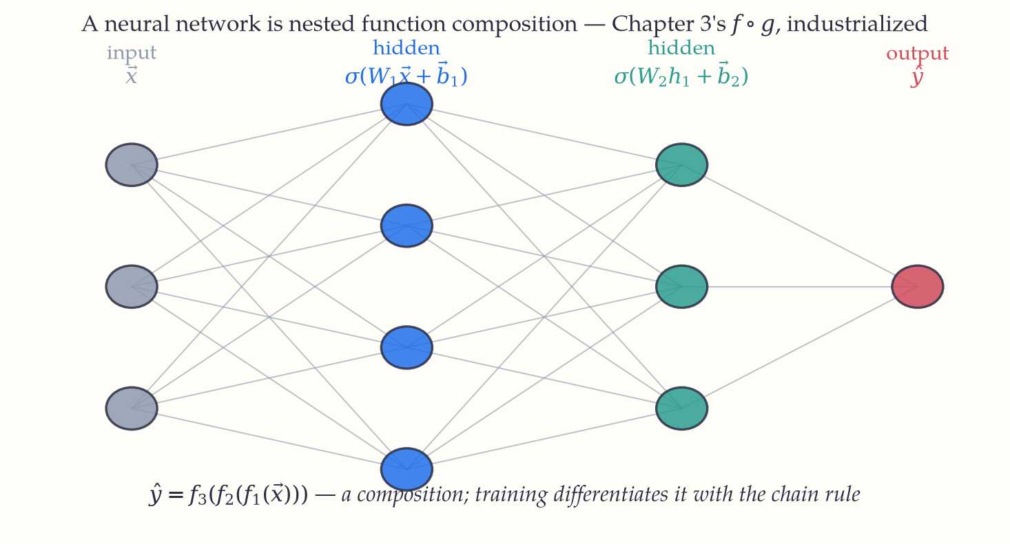
To improve a weight buried in layer 1, we need \frac{\partial L}{\partial W_1} — and Chapter 13 already told us how derivatives pass through compositions: they multiply along the chain.

\begin{gathered}\frac{\partial L}{\partial W_1} \\ = \frac{\partial L}{\partial f_3}\cdot\frac{\partial f_3}{\partial f_2}\cdot\frac{\partial f_2}{\partial f_1}\cdot\frac{\partial f_1}{\partial W_1}.\end{gathered}

Backpropagation is the bookkeeping that evaluates all such products efficiently — computing the loss forward through the network, then sweeping the derivatives backward, reusing shared factors so the whole gradient costs only about as much as one extra forward pass. Every deep-learning framework (PyTorch, TensorFlow, JAX) is, at its mathematical core, an automated chain rule. When a headline says a model was “trained on thousands of GPUs for months,” the computation being repeated is: chain rule, downhill step, chain rule, downhill step.

The chain-of-products form also explains deep learning’s classic ailments: many factors less than 1 multiply to nearly 0 (vanishing gradients — early layers stop learning), many factors above 1 explode. Cures like ReLU activations, careful initialization, and residual connections are all engineering responses to the arithmetic of long products.

Activation functions: why nonlinearity is non-negotiable#

Compose linear maps and you get a linear map (W_2(W_1\vec x) = (W_2W_1)\vec x) — a hundred stacked linear layers would collapse to one matrix. Intelligence requires bends. Between layers, networks insert a simple nonlinear activation:

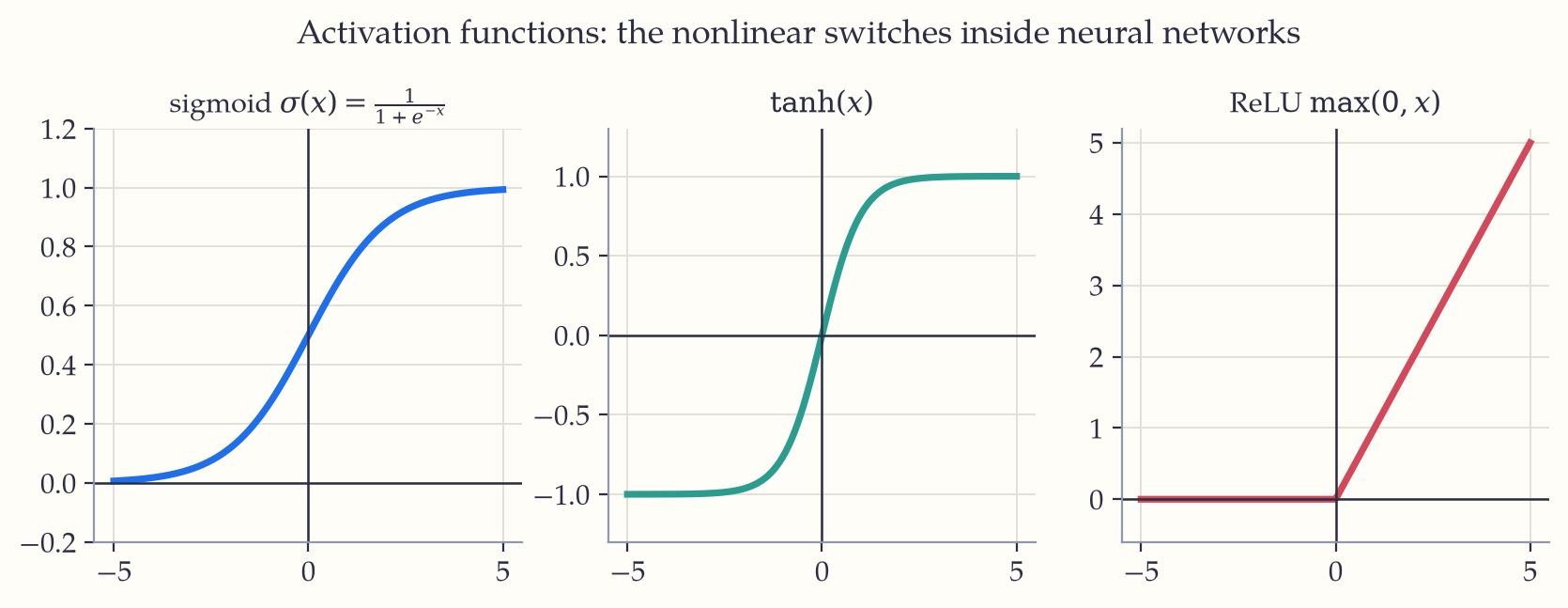
The sigmoid \sigma(x) = \frac{1}{1 + e^{-x}} squashes to (0,1) — Chapter 5’s exponential, arranged to output a probability; its derivative \sigma' = \sigma(1-\sigma) is a one-line exercise in the quotient rule. \tanh is its zero-centered sibling. ReLU = \max(0, x), almost insultingly simple, trains fastest in deep stacks precisely because its derivative is exactly 1 on the active side — long chain-rule products of 1s neither vanish nor explode. With any such nonlinearity, a wide enough network can approximate essentially any continuous function (the universal approximation theorem) — composition plus bends is expressively unlimited.

The shape of the landscape#

Whether descent finds the minimum or merely a minimum depends on the loss surface’s shape:

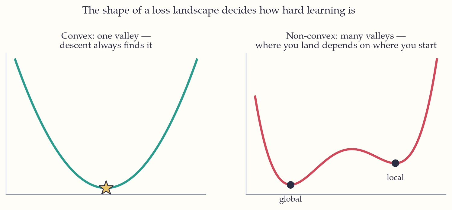
A convex function (bowl-shaped; the segment between any two points on the graph lies above the graph) has one global valley — descent cannot fail. Least squares and logistic regression are convex: their training is reliable and reproducible. Deep networks are gloriously non-convex, and that they train well anyway — in millions of dimensions, most critical points turn out to be saddles (Chapter 17) that stochastic descent slides off, and many local minima are nearly as good as the global one — is one of the field’s happiest empirical facts, and still an active research frontier.

If you keep one thing from this chapter: Learning is optimization: define a loss, step against the gradient at a sane learning rate, and let the chain rule — backpropagation — route the blame to every weight.